Manipulating Data with dplyr and tidyr
Last updated on 2026-04-24 | Edit this page
Overview
Questions
- How can I select specific rows and/or columns from a dataframe?
- How can I combine multiple commands into a single command?
- How can I create new columns or remove existing columns from a dataframe?
- How can I reformat a data frame to meet my needs?
Objectives
- Select certain columns in a dataframe with the
dplyrfunctionselect. - Select certain rows in a dataframe according to filtering conditions
with the
dplyrfunctionfilter. - Link the output of one
dplyrfunction to the input of another function with the ‘pipe’ operator%>%. - Add new columns to a dataframe that are functions of existing
columns with
mutate. - Use the split-apply-combine concept for data analysis.
- Use
summarize,group_by, andcountto split a dataframe into groups of observations, apply a summary statistics for each group, and then combine the results. - Describe the concept of a wide and a long table format and for which purpose those formats are useful.
- Describe the roles of variable names and their associated values when a table is reshaped.
- Reshape a dataframe from long to wide format and back with the
pivot_widerandpivot_longercommands from thetidyrpackage. - Export a dataframe to a
.csvfile.
dplyr is a package for making tabular
data wrangling easier by using a limited set of functions that can be
combined to extract and summarize insights from your data. It is a part
of the tidyverse, and is automatically loaded when you load the
tidyverse with libary(tidyverse).
dplyr pairs nicely with
tidyr which enables you to swiftly convert
between different data formats (long vs. wide) for plotting and
analysis.
Note
The packages in the tidyverse dplyr,
tidyr accept both the British
(e.g. summarise) and American (e.g. summarize)
spelling variants of different function and option names. For this
lesson, we utilize the American spellings of different functions;
however, feel free to use the regional variant for where you are
teaching.
To learn more about dplyr after this
workshop, you may want to check out this handy data transformation with **dplyr** cheatsheet.
To learn more about tidyr after the
workshop, you may want to check out this handy data tidying with **tidyr** cheatsheet.
Note
There are alternatives to the tidyverse packages for
data wrangling, including the package data.table.
See this comparison
for example to get a sense of the differences between using
base, tidyverse, and
data.table.
Acknowledgement
This workshop was adapted using material from the Data Carpentry
lessons R for Social Scientists,
specifically lesson 03-dplyr,
and lesson 04-tidyr
Other Materials
See Workshop 4 recording here - 1
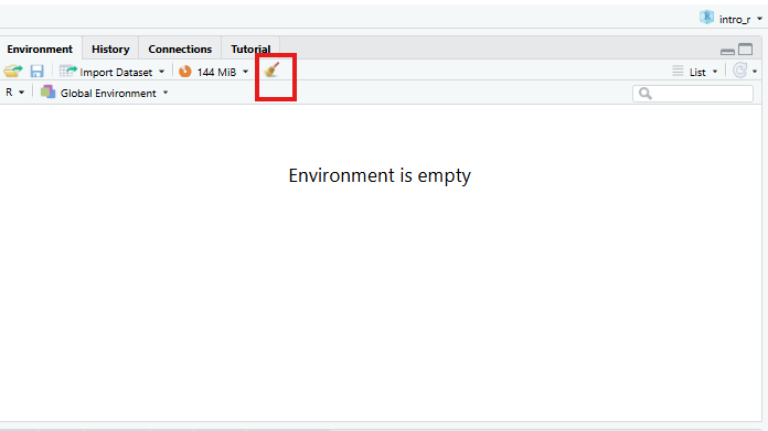
Set up
Start by opening up your RStudio project that you
created in a previous
workshop, called intro_r, in a new session. Ensure your
global environment is empty! You can also ‘sweep’ your
global environment by clicking the broom
icon.
Open a new R Notebook:
Click File -> New File -> R Notebook. Save your
R Notebook with a filename that makes sense, such as
manipulating_data.Rmd, in the scripts
folder.
When you open a new R Notebook, some explanatory text is
provided. This can be deleted so you can enter your own text and
code.
Read in the SAFI dataset that we downloaded earlier in a previous workshop.
R
## load the tidyverse
library(tidyverse)
library(here)

interviews <- read_csv(here("data", "raw", "SAFI_clean.csv"), na = "NULL")
interviews # preview the data
Learning dplyr
We’re going to learn some of the most common
dplyr functions:
-
select(): subset columns -
filter(): subset rows on conditions -
mutate(): create new columns by using information from other columns -
group_by()andsummarize(): create summary statistics on grouped data -
arrange(): sort results -
count(): count discrete values
Selecting columns and filtering rows
To select columns of a dataframe, use select(). The
first argument to this function is the dataframe
(interviews), and the subsequent arguments are the columns
to keep, separated by commas. Alternatively, if you are selecting
columns adjacent to each other, you can use a : to select a
range of columns, read as “select columns from ___ to ___.”
R
# to select columns throughout the dataframe
select(interviews, village, no_membrs, months_lack_food)
# to do the same thing with subsetting
interviews[c("village","no_membrs","months_lack_food")]
# to select a series of connected columns
select(interviews, village:respondent_wall_type)
To choose rows based on specific criteria, we can use the
filter() function. The argument after the dataframe is the
condition we want our final dataframe to adhere to (e.g. village name is
Chirodzo):
R
# filters observations where village name is "Chirodzo"
filter(interviews, village == "Chirodzo")
OUTPUT
# A tibble: 39 × 14
   key_ID village  interview_date      no_membrs years_liv respondent_wall_type
    <dbl> <chr>    <dttm>                  <dbl>     <dbl> <chr>
 1      8 Chirodzo 2016-11-16 00:00:00        12        70 burntbricks
 2      9 Chirodzo 2016-11-16 00:00:00         8         6 burntbricks
 3     10 Chirodzo 2016-12-16 00:00:00        12        23 burntbricks
 4     34 Chirodzo 2016-11-17 00:00:00         8        18 burntbricks
 5     35 Chirodzo 2016-11-17 00:00:00         5        45 muddaub
 6     36 Chirodzo 2016-11-17 00:00:00         6        23 sunbricks
 7     37 Chirodzo 2016-11-17 00:00:00         3         8 burntbricks
 8     43 Chirodzo 2016-11-17 00:00:00         7        29 muddaub
 9     44 Chirodzo 2016-11-17 00:00:00         2         6 muddaub
10     45 Chirodzo 2016-11-17 00:00:00         9         7 muddaub
# ℹ 29 more rows
# ℹ 8 more variables: rooms <dbl>, memb_assoc <chr>, affect_conflicts <chr>,
#   liv_count <dbl>, items_owned <chr>, no_meals <dbl>, months_lack_food <chr>,
#   instanceID <chr>
We can also specify multiple conditions within the
filter() function. We can combine conditions using either
“and” or “or” statements. In an “and” statement, an observation (row)
must meet every criteria to be included in the
resulting dataframe. To form “and” statements within dplyr, we can pass
our desired conditions as arguments in the filter()
function, separated by commas:
R
# filters observations with "and" operator (comma)
# output dataframe satisfies ALL specified conditions
filter(interviews, village == "Chirodzo",
                   rooms > 1,
                   no_meals > 2)
OUTPUT
# A tibble: 10 × 14
   key_ID village  interview_date      no_membrs years_liv respondent_wall_type
    <dbl> <chr>    <dttm>                  <dbl>     <dbl> <chr>
 1     10 Chirodzo 2016-12-16 00:00:00        12        23 burntbricks
 2     49 Chirodzo 2016-11-16 00:00:00         6        26 burntbricks
 3     52 Chirodzo 2016-11-16 00:00:00        11        15 burntbricks
 4     56 Chirodzo 2016-11-16 00:00:00        12        23 burntbricks
 5     65 Chirodzo 2016-11-16 00:00:00         8        20 burntbricks
 6     66 Chirodzo 2016-11-16 00:00:00        10        37 burntbricks
 7     67 Chirodzo 2016-11-16 00:00:00         5        31 burntbricks
 8     68 Chirodzo 2016-11-16 00:00:00         8        52 burntbricks
 9    199 Chirodzo 2017-06-04 00:00:00         7        17 burntbricks
10    200 Chirodzo 2017-06-04 00:00:00         8        20 burntbricks
# ℹ 8 more variables: rooms <dbl>, memb_assoc <chr>, affect_conflicts <chr>,
#   liv_count <dbl>, items_owned <chr>, no_meals <dbl>, months_lack_food <chr>,
#   instanceID <chr>
We can also form “and” statements with the &
operator instead of commas:
R
# filters observations with "&" logical operator
# output dataframe satisfies ALL specified conditions
filter(interviews, village == "Chirodzo" &
                   rooms > 1 &
                   no_meals > 2)
OUTPUT
# A tibble: 10 × 14
   key_ID village  interview_date      no_membrs years_liv respondent_wall_type
    <dbl> <chr>    <dttm>                  <dbl>     <dbl> <chr>
 1     10 Chirodzo 2016-12-16 00:00:00        12        23 burntbricks
 2     49 Chirodzo 2016-11-16 00:00:00         6        26 burntbricks
 3     52 Chirodzo 2016-11-16 00:00:00        11        15 burntbricks
 4     56 Chirodzo 2016-11-16 00:00:00        12        23 burntbricks
 5     65 Chirodzo 2016-11-16 00:00:00         8        20 burntbricks
 6     66 Chirodzo 2016-11-16 00:00:00        10        37 burntbricks
 7     67 Chirodzo 2016-11-16 00:00:00         5        31 burntbricks
 8     68 Chirodzo 2016-11-16 00:00:00         8        52 burntbricks
 9    199 Chirodzo 2017-06-04 00:00:00         7        17 burntbricks
10    200 Chirodzo 2017-06-04 00:00:00         8        20 burntbricks
# ℹ 8 more variables: rooms <dbl>, memb_assoc <chr>, affect_conflicts <chr>,
#   liv_count <dbl>, items_owned <chr>, no_meals <dbl>, months_lack_food <chr>,
#   instanceID <chr>
In an “or” statement, observations must meet at least one of the specified conditions. To form “or” statements we use the logical operator for “or,” which is the vertical bar (|):
R
# filters observations with "|" logical operator
# output dataframe satisfies AT LEAST ONE of the specified conditions
filter(interviews, village == "Chirodzo" | village == "Ruaca")
OUTPUT
# A tibble: 88 × 14
   key_ID village  interview_date      no_membrs years_liv respondent_wall_type
    <dbl> <chr>    <dttm>                  <dbl>     <dbl> <chr>
 1      8 Chirodzo 2016-11-16 00:00:00        12        70 burntbricks
 2      9 Chirodzo 2016-11-16 00:00:00         8         6 burntbricks
 3     10 Chirodzo 2016-12-16 00:00:00        12        23 burntbricks
 4     23 Ruaca    2016-11-21 00:00:00        10        20 burntbricks
 5     24 Ruaca    2016-11-21 00:00:00         6         4 burntbricks
 6     25 Ruaca    2016-11-21 00:00:00        11         6 burntbricks
 7     26 Ruaca    2016-11-21 00:00:00         3        20 burntbricks
 8     27 Ruaca    2016-11-21 00:00:00         7        36 burntbricks
 9     28 Ruaca    2016-11-21 00:00:00         2         2 muddaub
10     29 Ruaca    2016-11-21 00:00:00         7        10 burntbricks
# ℹ 78 more rows
# ℹ 8 more variables: rooms <dbl>, memb_assoc <chr>, affect_conflicts <chr>,
#   liv_count <dbl>, items_owned <chr>, no_meals <dbl>, months_lack_food <chr>,
#   instanceID <chr>
Pipes
What if you want to select and filter at the same time? There are three ways to do this: use intermediate steps, nested functions, or pipes.
With intermediate steps, you create a temporary dataframe and use that as input to the next function, like this:
R
interviews2 <- filter(interviews, village == "Chirodzo")
interviews_ch <- select(interviews2, village:respondent_wall_type)
This is readable, but can clutter up your workspace with lots of objects that you have to name individually. With multiple steps, that can be hard to keep track of.
You can also nest functions (i.e. one function inside of another), like this:
R
interviews_ch <- select(filter(interviews, village == "Chirodzo"),
                         village:respondent_wall_type)
This is handy, but can be difficult to read if too many functions are
nested, as R evaluates the expression from the inside out
(in this case, filtering, then selecting).
The last option are pipes. Pipes let you take the output of
one function and send it directly to the next, which is useful when you
need to do many things to the same dataset. We’ll use the
tidyverse pipe %>% which can be typed
with:
Ctrl+Shift+M (Windows and
Linux) or Cmd+Shift+M
(Mac).
R
# the following example is run using magrittr pipe but the output will be same with the native pipe
interviews %>%
    filter(village == "Chirodzo") %>%
    select(village:respondent_wall_type)
OUTPUT
# A tibble: 39 × 5
   village  interview_date      no_membrs years_liv respondent_wall_type
   <chr>    <dttm>                  <dbl>     <dbl> <chr>
 1 Chirodzo 2016-11-16 00:00:00        12        70 burntbricks
 2 Chirodzo 2016-11-16 00:00:00         8         6 burntbricks
 3 Chirodzo 2016-12-16 00:00:00        12        23 burntbricks
 4 Chirodzo 2016-11-17 00:00:00         8        18 burntbricks
 5 Chirodzo 2016-11-17 00:00:00         5        45 muddaub
 6 Chirodzo 2016-11-17 00:00:00         6        23 sunbricks
 7 Chirodzo 2016-11-17 00:00:00         3         8 burntbricks
 8 Chirodzo 2016-11-17 00:00:00         7        29 muddaub
 9 Chirodzo 2016-11-17 00:00:00         2         6 muddaub
10 Chirodzo 2016-11-17 00:00:00         9         7 muddaub
# ℹ 29 more rows
R
#interviews |>
#   filter(village == "Chirodzo") |>
#   select(village:respondent_wall_type)
In the above code, we use the pipe to send the
interviews dataset first through filter() to
keep rows where village is Chirodzo, then
through select() to keep only the columns from
village to respondent_wall_type. Since
%>% takes the object on its left and passes it as the
first argument to the function on its right, we don’t need to explicitly
include the dataframe as an argument to the filter() and
select() functions any more.
Some may find it helpful to read the pipe like the word “then”. For
instance, in the above example, we take the dataframe
interviews, then we filter for rows
with village == "Chirodzo", then we
select columns village:respondent_wall_type.
The dplyr functions by themselves are
somewhat simple, but by combining them into linear workflows with the
pipe, we can accomplish more complex data wrangling operations.
If we want to create a new object with this smaller version of the data, we can assign it a new name:
R
interviews_ch <- interviews %>%
    filter(village == "Chirodzo") %>%
    select(village:respondent_wall_type)

interviews_ch
OUTPUT
# A tibble: 39 × 5
   village  interview_date      no_membrs years_liv respondent_wall_type
   <chr>    <dttm>                  <dbl>     <dbl> <chr>
 1 Chirodzo 2016-11-16 00:00:00        12        70 burntbricks
 2 Chirodzo 2016-11-16 00:00:00         8         6 burntbricks
 3 Chirodzo 2016-12-16 00:00:00        12        23 burntbricks
 4 Chirodzo 2016-11-17 00:00:00         8        18 burntbricks
 5 Chirodzo 2016-11-17 00:00:00         5        45 muddaub
 6 Chirodzo 2016-11-17 00:00:00         6        23 sunbricks
 7 Chirodzo 2016-11-17 00:00:00         3         8 burntbricks
 8 Chirodzo 2016-11-17 00:00:00         7        29 muddaub
 9 Chirodzo 2016-11-17 00:00:00         2         6 muddaub
10 Chirodzo 2016-11-17 00:00:00         9         7 muddaub
# ℹ 29 more rows
Note that the final dataframe (interviews_ch) is the
leftmost part of this expression.
Exercise
Using pipes, subset the interviews data to include
interviews where respondents were members of an irrigation association
(memb_assoc) and retain only the columns
affect_conflicts, liv_count, and
no_meals.
R
interviews %>%
    filter(memb_assoc == "yes") %>%
    select(affect_conflicts, liv_count, no_meals)
OUTPUT
# A tibble: 33 × 3
   affect_conflicts liv_count no_meals
   <chr>                <dbl>    <dbl>
 1 once                     3        2
 2 never                    2        2
 3 never                    2        3
 4 once                     3        2
 5 frequently               1        3
 6 more_once                5        2
 7 more_once                3        2
 8 more_once                2        3
 9 once                     3        3
10 never                    3        3
# ℹ 23 more rows
Mutate
Frequently you’ll want to create new columns based on the values in
existing columns, for example to do unit conversions, or to find the
ratio of values in two columns. For this we’ll use
mutate().
We might be interested in the ratio of number of household members to rooms used for sleeping (i.e. the average number of people per room):
R
interviews %>%
    mutate(people_per_room = no_membrs / rooms)
OUTPUT
# A tibble: 131 × 15
   key_ID village  interview_date      no_membrs years_liv respondent_wall_type
    <dbl> <chr>    <dttm>                  <dbl>     <dbl> <chr>
 1      1 God      2016-11-17 00:00:00         3         4 muddaub
 2      2 God      2016-11-17 00:00:00         7         9 muddaub
 3      3 God      2016-11-17 00:00:00        10        15 burntbricks
 4      4 God      2016-11-17 00:00:00         7         6 burntbricks
 5      5 God      2016-11-17 00:00:00         7        40 burntbricks
 6      6 God      2016-11-17 00:00:00         3         3 muddaub
 7      7 God      2016-11-17 00:00:00         6        38 muddaub
 8      8 Chirodzo 2016-11-16 00:00:00        12        70 burntbricks
 9      9 Chirodzo 2016-11-16 00:00:00         8         6 burntbricks
10     10 Chirodzo 2016-12-16 00:00:00        12        23 burntbricks
# ℹ 121 more rows
# ℹ 9 more variables: rooms <dbl>, memb_assoc <chr>, affect_conflicts <chr>,
#   liv_count <dbl>, items_owned <chr>, no_meals <dbl>, months_lack_food <chr>,
#   instanceID <chr>, people_per_room <dbl>
We may be interested in investigating whether being a member of an
irrigation association had any effect on the ratio of household members
to rooms. To look at this relationship, we will first remove data from
our dataset where the respondent didn’t answer the question of whether
they were a member of an irrigation association. These cases are
recorded as NULL in the dataset.
To remove these cases, we could insert a filter() in the
chain:
R
interviews %>%
    filter(!is.na(memb_assoc)) %>%
    mutate(people_per_room = no_membrs / rooms)
OUTPUT
# A tibble: 92 × 15
   key_ID village  interview_date      no_membrs years_liv respondent_wall_type
    <dbl> <chr>    <dttm>                  <dbl>     <dbl> <chr>
 1      2 God      2016-11-17 00:00:00         7         9 muddaub
 2      7 God      2016-11-17 00:00:00         6        38 muddaub
 3      8 Chirodzo 2016-11-16 00:00:00        12        70 burntbricks
 4      9 Chirodzo 2016-11-16 00:00:00         8         6 burntbricks
 5     10 Chirodzo 2016-12-16 00:00:00        12        23 burntbricks
 6     12 God      2016-11-21 00:00:00         7        20 burntbricks
 7     13 God      2016-11-21 00:00:00         6         8 burntbricks
 8     15 God      2016-11-21 00:00:00         5        30 sunbricks
 9     21 God      2016-11-21 00:00:00         8        20 burntbricks
10     24 Ruaca    2016-11-21 00:00:00         6         4 burntbricks
# ℹ 82 more rows
# ℹ 9 more variables: rooms <dbl>, memb_assoc <chr>, affect_conflicts <chr>,
#   liv_count <dbl>, items_owned <chr>, no_meals <dbl>, months_lack_food <chr>,
#   instanceID <chr>, people_per_room <dbl>
The ! symbol negates the result of the
is.na() function. Thus, if is.na() returns a
value of TRUE (because the memb_assoc is
missing), the ! symbol negates this and says we only want
values of FALSE, where memb_assoc is
not missing.
Exercise
Create a new dataframe from the interviews data that
meets the following criteria: contains only the village
column and a new column called total_meals containing a
value that is equal to the total number of meals served in the household
per day on average (no_membrs times no_meals).
Only the rows where total_meals is greater than 20 should
be shown in the final dataframe.
Hint: think about how the commands should be ordered to produce this data frame!
R
interviews_total_meals <- interviews %>%
    mutate(total_meals = no_membrs * no_meals) %>%
    filter(total_meals > 20) %>%
    select(village, total_meals)
Split-apply-combine data analysis and the
summarize() function
Many data analysis tasks can be approached using the
split-apply-combine paradigm: split the data into
groups, apply some analysis to each group, and then combine the results.
dplyr makes this very easy through the use
of the group_by() function.
The summarize() function
group_by() is often used together with
summarize(), which collapses each group into a single-row
summary of that group. group_by() takes as arguments the
column names that contain the categorical variables for
which you want to calculate the summary statistics. So to compute the
average household size by village:
R
interviews %>%
    group_by(village) %>%
    summarize(mean_no_membrs = mean(no_membrs))
OUTPUT
# A tibble: 3 × 2
  village  mean_no_membrs
  <chr>             <dbl>
1 Chirodzo           7.08
2 God                6.86
3 Ruaca              7.57
You can also group by multiple columns:
R
interviews %>%
    group_by(village, memb_assoc) %>%
    summarize(mean_no_membrs = mean(no_membrs))
OUTPUT
`summarise()` has regrouped the output.
ℹ Summaries were computed grouped by village and memb_assoc.
ℹ Output is grouped by village.
ℹ Use `summarise(.groups = "drop_last")` to silence this message.
ℹ Use `summarise(.by = c(village, memb_assoc))` for per-operation grouping
  (`?dplyr::dplyr_by`) instead.
OUTPUT
# A tibble: 9 × 3
# Groups:   village [3]
  village  memb_assoc mean_no_membrs
  <chr>    <chr>               <dbl>
1 Chirodzo no                   8.06
2 Chirodzo yes                  7.82
3 Chirodzo <NA>                 5.08
4 God      no                   7.13
5 God      yes                  8
6 God      <NA>                 6
7 Ruaca    no                   7.18
8 Ruaca    yes                  9.5
9 Ruaca    <NA>                 6.22
Note that the output is a grouped tibble of nine rows by three
columns which is indicated by the by two first lines with the
#. To obtain an ungrouped tibble, use the
ungroup function:
R
interviews %>%
    group_by(village, memb_assoc) %>%
    summarize(mean_no_membrs = mean(no_membrs)) %>%
    ungroup()
OUTPUT
`summarise()` has regrouped the output.
ℹ Summaries were computed grouped by village and memb_assoc.
ℹ Output is grouped by village.
ℹ Use `summarise(.groups = "drop_last")` to silence this message.
ℹ Use `summarise(.by = c(village, memb_assoc))` for per-operation grouping
  (`?dplyr::dplyr_by`) instead.
OUTPUT
# A tibble: 9 × 3
  village  memb_assoc mean_no_membrs
  <chr>    <chr>               <dbl>
1 Chirodzo no                   8.06
2 Chirodzo yes                  7.82
3 Chirodzo <NA>                 5.08
4 God      no                   7.13
5 God      yes                  8
6 God      <NA>                 6
7 Ruaca    no                   7.18
8 Ruaca    yes                  9.5
9 Ruaca    <NA>                 6.22
Notice that the second line with the # that previously
indicated the grouping has disappeared and we now only have a 9x3-tibble
without grouping. When grouping both by village and
membr_assoc, we see rows in our table for respondents who
did not specify whether they were a member of an irrigation association.
We can exclude those data from our table using a filter step.
R
interviews %>%
    filter(!is.na(memb_assoc)) %>%
    group_by(village, memb_assoc) %>%
    summarize(mean_no_membrs = mean(no_membrs))
OUTPUT
`summarise()` has regrouped the output.
ℹ Summaries were computed grouped by village and memb_assoc.
ℹ Output is grouped by village.
ℹ Use `summarise(.groups = "drop_last")` to silence this message.
ℹ Use `summarise(.by = c(village, memb_assoc))` for per-operation grouping
  (`?dplyr::dplyr_by`) instead.
OUTPUT
# A tibble: 6 × 3
# Groups:   village [3]
  village  memb_assoc mean_no_membrs
  <chr>    <chr>               <dbl>
1 Chirodzo no                   8.06
2 Chirodzo yes                  7.82
3 God      no                   7.13
4 God      yes                  8
5 Ruaca    no                   7.18
6 Ruaca    yes                  9.5
Once the data are grouped, you can also summarize multiple variables at the same time (and not necessarily on the same variable). For instance, we could add a column indicating the minimum household size for each village for each group (members of an irrigation association vs not):
R
interviews %>%
    filter(!is.na(memb_assoc)) %>%
    group_by(village, memb_assoc) %>%
    summarize(mean_no_membrs = mean(no_membrs),
              min_membrs = min(no_membrs))
OUTPUT
`summarise()` has regrouped the output.
ℹ Summaries were computed grouped by village and memb_assoc.
ℹ Output is grouped by village.
ℹ Use `summarise(.groups = "drop_last")` to silence this message.
ℹ Use `summarise(.by = c(village, memb_assoc))` for per-operation grouping
  (`?dplyr::dplyr_by`) instead.
OUTPUT
# A tibble: 6 × 4
# Groups:   village [3]
  village  memb_assoc mean_no_membrs min_membrs
  <chr>    <chr>               <dbl>      <dbl>
1 Chirodzo no                   8.06          4
2 Chirodzo yes                  7.82          2
3 God      no                   7.13          3
4 God      yes                  8             5
5 Ruaca    no                   7.18          2
6 Ruaca    yes                  9.5           5
It is sometimes useful to rearrange the result of a query to inspect
the values. For instance, we can sort on min_membrs to put
the group with the smallest household first:
R
interviews %>%
    filter(!is.na(memb_assoc)) %>%
    group_by(village, memb_assoc) %>%
    summarize(mean_no_membrs = mean(no_membrs),
              min_membrs = min(no_membrs)) %>%
    arrange(min_membrs)
OUTPUT
`summarise()` has regrouped the output.
ℹ Summaries were computed grouped by village and memb_assoc.
ℹ Output is grouped by village.
ℹ Use `summarise(.groups = "drop_last")` to silence this message.
ℹ Use `summarise(.by = c(village, memb_assoc))` for per-operation grouping
  (`?dplyr::dplyr_by`) instead.
OUTPUT
# A tibble: 6 × 4
# Groups:   village [3]
  village  memb_assoc mean_no_membrs min_membrs
  <chr>    <chr>               <dbl>      <dbl>
1 Chirodzo yes                  7.82          2
2 Ruaca    no                   7.18          2
3 God      no                   7.13          3
4 Chirodzo no                   8.06          4
5 God      yes                  8             5
6 Ruaca    yes                  9.5           5
To sort in descending order, we need to add the desc()
function. If we want to sort the results by decreasing order of minimum
household size:
R
interviews %>%
    filter(!is.na(memb_assoc)) %>%
    group_by(village, memb_assoc) %>%
    summarize(mean_no_membrs = mean(no_membrs),
              min_membrs = min(no_membrs)) %>%
    arrange(desc(min_membrs))
OUTPUT
`summarise()` has regrouped the output.
ℹ Summaries were computed grouped by village and memb_assoc.
ℹ Output is grouped by village.
ℹ Use `summarise(.groups = "drop_last")` to silence this message.
ℹ Use `summarise(.by = c(village, memb_assoc))` for per-operation grouping
  (`?dplyr::dplyr_by`) instead.
OUTPUT
# A tibble: 6 × 4
# Groups:   village [3]
  village  memb_assoc mean_no_membrs min_membrs
  <chr>    <chr>               <dbl>      <dbl>
1 God      yes                  8             5
2 Ruaca    yes                  9.5           5
3 Chirodzo no                   8.06          4
4 God      no                   7.13          3
5 Chirodzo yes                  7.82          2
6 Ruaca    no                   7.18          2
Counting
When working with data, we often want to know the number of
observations found for each factor or combination of factors. For this
task, dplyr provides count().
For example, if we wanted to count the number of rows of data for each
village, we would do:
R
interviews %>%
    count(village)
OUTPUT
# A tibble: 3 × 2
  village      n
  <chr>    <int>
1 Chirodzo    39
2 God         43
3 Ruaca       49
For convenience, count() provides the sort
argument to get results in decreasing order:
R
interviews %>%
    count(village, sort = TRUE)
OUTPUT
# A tibble: 3 × 2
  village      n
  <chr>    <int>
1 Ruaca       49
2 God         43
3 Chirodzo 39Exercise
How many households in the survey have an average of two meals per day? Three meals per day? Are there any other numbers of meals represented?
R
interviews %>%
   count(no_meals)
OUTPUT
# A tibble: 2 × 2
  no_meals     n
     <dbl> <int>
1        2    52
2 3 79Exercise (continued)
Use group_by() and summarize() to find the
mean, min, and max number of household members for each village. Also
add the number of observations (hint: see ?n).
R
interviews %>%
  group_by(village) %>%
  summarize(
      mean_no_membrs = mean(no_membrs),
      min_no_membrs = min(no_membrs),
      max_no_membrs = max(no_membrs),
      n = n()
  )
OUTPUT
# A tibble: 3 × 5
  village  mean_no_membrs min_no_membrs max_no_membrs     n
  <chr>             <dbl>         <dbl>         <dbl> <int>
1 Chirodzo           7.08             2            12    39
2 God                6.86             3            15    43
3 Ruaca 7.57 2 19 49Exercise (continued)
What was the largest household interviewed in each month?
R
# if not already included, add month, year, and day columns
library(lubridate) # load lubridate if not already loaded
interviews %>%
    mutate(month = month(interview_date),
           day = day(interview_date),
           year = year(interview_date)) %>%
    group_by(year, month) %>%
    summarize(max_no_membrs = max(no_membrs))
OUTPUT
`summarise()` has regrouped the output.
ℹ Summaries were computed grouped by year and month.
ℹ Output is grouped by year.
ℹ Use `summarise(.groups = "drop_last")` to silence this message.
ℹ Use `summarise(.by = c(year, month))` for per-operation grouping
  (`?dplyr::dplyr_by`) instead.
OUTPUT
# A tibble: 5 × 3
# Groups:   year [2]
   year month max_no_membrs
  <dbl> <dbl>         <dbl>
1  2016    11            19
2  2016    12            12
3  2017     4            17
4  2017     5            15
5  2017     6            15
Learning tidyr
Reshaping with pivot_wider() and
pivot_longer()
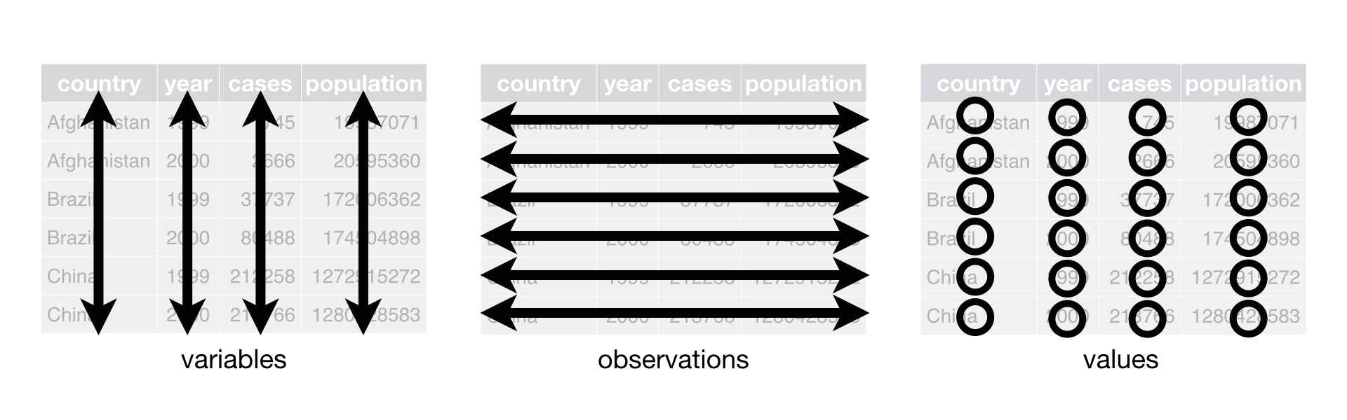
There are essentially three rules that define a “tidy” dataset:
- Each variable has its own column
- Each observation has its own row
- Each value must have its own cell
This graphic visually represents the three rules that define a “tidy” dataset:
 R for Data Science,
Wickham H and Grolemund G (https://r4ds.had.co.nz/index.html) © Wickham, Grolemund
2017 This image is licenced under Attribution-NonCommercial-NoDerivs 3.0
United States (CC-BY-NC-ND 3.0 US)
R for Data Science,
Wickham H and Grolemund G (https://r4ds.had.co.nz/index.html) © Wickham, Grolemund
2017 This image is licenced under Attribution-NonCommercial-NoDerivs 3.0
United States (CC-BY-NC-ND 3.0 US)
In this section we will explore how these rules are linked to the
different data formats researchers are often interested in: “wide” and
“long”. This tutorial will help you efficiently transform your data
shape regardless of original format. First we will explore qualities of
the interviews data and how they relate to these different
types of data formats.
Long and wide data formats
In the interviews data, each row contains the values of
variables associated with each record collected (each interview in the
villages). It is stated that the key_ID was “added to
provide a unique Id for each observation” and the
instanceID “does this as well but it is not as convenient
to use.”
Once we have established that key_ID and
instanceID are both unique we can use either variable as an
identifier corresponding to the 131 interview records.
R
interviews %>%
  select(key_ID) %>%
  distinct() %>%
  nrow()
OUTPUT
[1] 131As seen in the code below, for each interview date in each village no
instanceIDs are the same. Thus, this format is what is
called a “long” data format, where each observation occupies only one
row in the dataframe.
R
interviews %>%
  filter(village == "Chirodzo") %>%
  select(key_ID, village, interview_date, instanceID) %>%
  sample_n(size = 10)
OUTPUT
# A tibble: 10 × 4
   key_ID village  interview_date      instanceID
    <dbl> <chr>    <dttm>              <chr>
 1     57 Chirodzo 2016-11-16 00:00:00 uuid:a7184e55-0615-492d-9835-8f44f3b03a71
 2     10 Chirodzo 2016-12-16 00:00:00 uuid:8f4e49bc-da81-4356-ae34-e0d794a23721
 3     53 Chirodzo 2016-11-16 00:00:00 uuid:cc7f75c5-d13e-43f3-97e5-4f4c03cb4b12
 4     34 Chirodzo 2016-11-17 00:00:00 uuid:14c78c45-a7cc-4b2a-b765-17c82b43feb4
 5     59 Chirodzo 2016-11-16 00:00:00 uuid:1936db62-5732-45dc-98ff-9b3ac7a22518
 6     65 Chirodzo 2016-11-16 00:00:00 uuid:143f7478-0126-4fbc-86e0-5d324339206b
 7    199 Chirodzo 2017-06-04 00:00:00 uuid:ffc83162-ff24-4a87-8709-eff17abc0b3b
 8     51 Chirodzo 2016-11-16 00:00:00 uuid:18ac8e77-bdaf-47ab-85a2-e4c947c9d3ce
 9    192 Chirodzo 2017-06-03 00:00:00 uuid:f94409a6-e461-4e4c-a6fb-0072d3d58b00
10    200 Chirodzo 2017-06-04 00:00:00 uuid:aa77a0d7-7142-41c8-b494-483a5b68d8a7
We notice that the layout or format of the interviews
data is in a format that adheres to rules 1-3, where
- each column is a variable
- each row is an observation
- each value has its own cell
This is called a “long” data format. But, we notice that each column represents a different variable. In the “longest” data format there would only be three columns, one for the id variable, one for the observed variable, and one for the observed value (of that variable). This data format is quite unsightly and difficult to work with, so you will rarely see it in use.
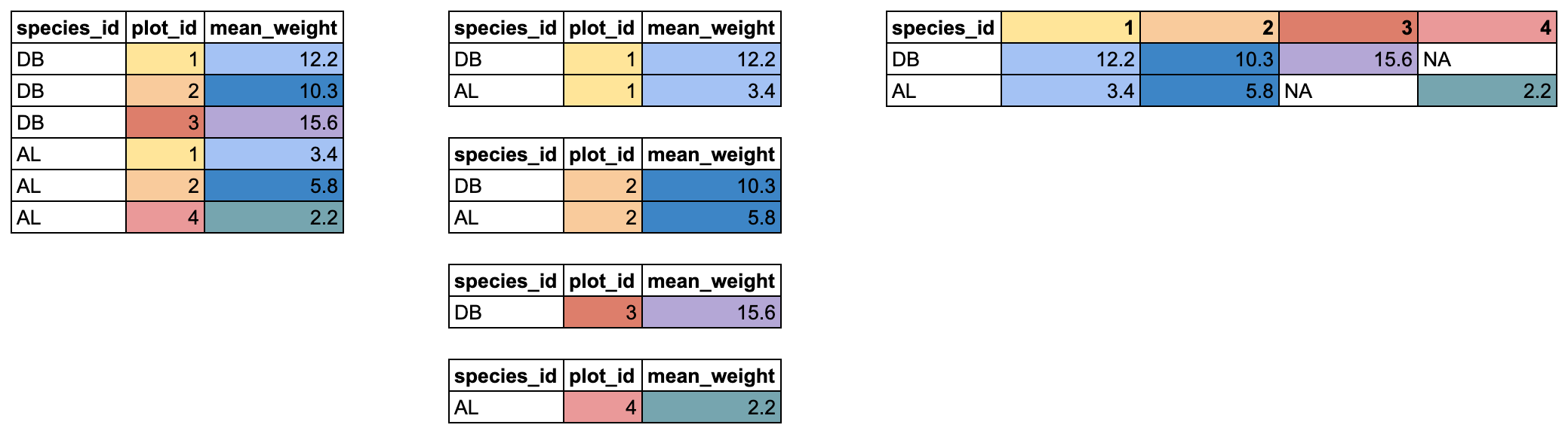
Alternatively, in a “wide” data format we see modifications to rule 1, where each column no longer represents a single variable. Instead, columns can represent different levels/values of a variable. For instance, in some data you encounter the researchers may have chosen for every survey date to be a different column.
These may sound like dramatically different data layouts, but there
are some tools that make transitions between these layouts much simpler
than you might think! The gif below shows how these two
formats relate to each other, and gives you an idea of how we can use
R to shift from one format to the other.
Long and wide dataframe layouts mainly affect readability. You may
find that visually you may prefer the “wide” format, since you can see
more of the data on the screen. However, all of the R
functions we have used thus far expect for your data to be in a “long”
data format. This is because the long format is more machine readable
and is closer to the formatting of databases.
Questions which warrant different data formats
In interviews, each row contains the values of variables associated with each record (the unit), values such as the village of the respondent, the number of household members, or the type of wall their house had. This format allows for us to make comparisons across individual surveys, but what if we wanted to look at differences in households grouped by different types of items owned?
To facilitate this comparison we would need to create a new table
where each row (the unit) was comprised of values of variables
associated with items owned (i.e., items_owned). In
practical terms this means the values of the items in
items_owned (e.g. bicycle, radio, table, etc.) would become
the names of column variables and the cells would contain values of
TRUE or FALSE, for whether that household had
that item.
Once we we’ve created this new table, we can explore the relationship within and between villages. The key point here is that we are still following a tidy data structure, but we have reshaped the data according to the observations of interest.
Alternatively, if the interview dates were spread across multiple columns, and we were interested in visualizing, within each village, how irrigation conflicts have changed over time. This would require for the interview date to be included in a single column rather than spread across multiple columns. Thus, we would need to transform the column names into values of a variable.
We can do both of these transformations with two tidyr
functions, pivot_wider() and
pivot_longer().
Pivoting wider
pivot_wider() takes three principal arguments:
- the
data - the
names_fromcolumn variable whose values will become new column names. - the
values_fromcolumn variable whose values will fill the new column variables.
Further arguments include values_fill which, if set,
fills in missing values with the value provided.
Let’s use pivot_wider() to transform interviews to
create new columns for each item owned by a household. There are a
couple of new concepts in this transformation, so let’s walk through it
line by line. First we create a new object
(interviews_items_owned) based on the
interviews data frame.
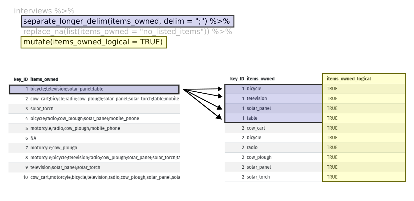
Then we will actually need to make our data frame longer, because we
have multiple items in a single cell. We will use a new function,
separate_longer_delim(), from the
tidyr package to separate the values of
items_owned based on the presence of semi-colons
(;). The values of this variable were multiple items
separated by semi-colons, so this action creates a row for each item
listed in a household’s possession. Thus, we end up with a long format
version of the dataset, with multiple rows for each respondent. For
example, if a respondent has a television and a solar panel, that
respondent will now have two rows, one with “television” and the other
with “solar panel” in the items_owned column.
After this transformation, you may notice that the
items_owned column contains NA values. This is
because some of the respondents did not own any of the items in the
interviewer’s list. We can use the replace_na() function to
change these NA values to something more meaningful. The
replace_na() function expects for you to give it a
list() of columns that you would like to replace the
NA values in, and the value that you would like to replace
the NAs. This ends up looking like this:
Next, we create a new variable named
items_owned_logical, which has one value
(TRUE) for every row. This makes sense, since each item in
every row was owned by that household. We are constructing this variable
so that when we spread the items_owned across multiple
columns, we can fill the values of those columns with logical values
describing whether the household did (TRUE) or did not
(FALSE) own that particular item.
At this point, we can also count the number of items owned by each
household, which is equivalent to the number of rows per
key_ID. We can do this with a group_by() and
mutate() pipeline that works similar to
group_by() and summarize() discussed in the
previous episode but instead of creating a summary table, we will add
another column called number_items. We use the
n() function to count the number of rows within each group.
However, there is one difficulty we need to take into account, namely
those households that did not list any items. These households now have
"no_listed_items" under items_owned. We do not
want to count this as an item but instead show zero items. We can
accomplish this using dplyr’s
if_else() function that evaluates a condition and returns
one value if true and another if false. Here, if the
items_owned column is "no_listed_items", then
a 0 is returned, otherwise, the number of rows per group is returned
using n().
Lastly, we use pivot_wider() to switch from long format
to wide format. This creates a new column for each of the unique values
in the items_owned column, and fills those columns with the
values of items_owned_logical. We also declare that for
items that are missing, we want to fill those cells with the value of
FALSE instead of NA.
R
pivot_wider(names_from = items_owned,
            values_from = items_owned_logical,
            values_fill = list(items_owned_logical = FALSE))
Combining the above steps, the chunk looks like this. Note that two
new columns are created within the same mutate() call.
R
interviews_items_owned <- interviews %>%
  separate_longer_delim(items_owned, delim = ";") %>%
  replace_na(list(items_owned = "no_listed_items")) %>%
  group_by(key_ID) %>%
  mutate(items_owned_logical = TRUE,
         number_items = if_else(items_owned == "no_listed_items", 0, n())) %>%
  pivot_wider(names_from = items_owned,
              values_from = items_owned_logical,
              values_fill = list(items_owned_logical = FALSE))
View the interviews_items_owned data frame. It should
have 131 rows (the same number of rows you had originally), but extra
columns for each item. How many columns were added? Notice that there is
no longer a column titled items_owned. This is because
there is a default parameter in pivot_wider() that drops
the original column. The values that were in that column have now become
columns named television, solar_panel,
table, etc. You can use dim(interviews) and
dim(interviews_wide) to see how the number of columns has
changed between the two datasets.
This format of the data allows us to do interesting things, like make a table showing the number of respondents in each village who owned a particular item:
R
interviews_items_owned %>%
  filter(bicycle) %>%
  group_by(village) %>%
  count(bicycle)
OUTPUT
# A tibble: 3 × 3
# Groups:   village [3]
  village  bicycle     n
  <chr>    <lgl>   <int>
1 Chirodzo TRUE       17
2 God      TRUE       23
3 Ruaca    TRUE       20
Or below we calculate the average number of items from the list owned
by respondents in each village using the number_items
column we created to count the items listed by each household.
R
interviews_items_owned %>%
    group_by(village) %>%
    summarize(mean_items = mean(number_items))
OUTPUT
# A tibble: 3 × 2
  village  mean_items
  <chr>         <dbl>
1 Chirodzo       4.54
2 God            3.98
3 Ruaca 5.57Exercise
We created interviews_items_owned by reshaping the data:
first longer and then wider. Replicate this process with the
months_lack_food column in the interviews
dataframe. Create a new dataframe with columns for each of the months
filled with logical vectors (TRUE or FALSE)
and a summary column called number_months_lack_food that
calculates the number of months each household reported a lack of
food.
Note that if the household did not lack food in the previous 12
months, the value input was none.
R
months_lack_food <- interviews %>%
  separate_longer_delim(months_lack_food, delim = ";") %>%
  group_by(key_ID) %>%
  mutate(months_lack_food_logical = TRUE,
         number_months_lack_food = if_else(months_lack_food == "none", 0, n())) %>%
  pivot_wider(names_from = months_lack_food,
              values_from = months_lack_food_logical,
              values_fill = list(months_lack_food_logical = FALSE))
Pivoting longer
The opposing situation could occur if we had been provided with data
in the form of interviews_wide, where the items owned are
column names, but we wish to treat them as values of an
items_owned variable instead.
In this situation we are gathering these columns turning them into a pair of new variables. One variable includes the column names as values, and the other variable contains the values in each cell previously associated with the column names. We will do this in two steps to make this process a bit clearer.
pivot_longer() takes four principal arguments:
- the
data -
colsare the names of the columns we use to fill the a new values variable (or to drop). - the
names_tocolumn variable we wish to create from thecolsprovided. - the
values_tocolumn variable we wish to create and fill with values associated with thecolsprovided.
R
interviews_long <- interviews_items_owned %>%
  pivot_longer(cols = bicycle:car,
               names_to = "items_owned",
               values_to = "items_owned_logical")
View both interviews_long and
interviews_items_owned and compare their structure.
Exercise
We created some summary tables on interviews_items_owned
using count and summarise. We can create the
same tables on interviews_long, but this will require a
different process.
Make a table showing the number of respondents in each village who
owned a particular item, and include all items. The difference between
this format and the wide format is that you can now count
all the items using the items_owned variable.
R
interviews_long %>%
  filter(items_owned_logical) %>%
  group_by(village) %>%
  count(items_owned)
OUTPUT
# A tibble: 47 × 3
# Groups:   village [3]
   village  items_owned         n
   <chr>    <chr>           <int>
 1 Chirodzo bicycle            17
 2 Chirodzo computer            2
 3 Chirodzo cow_cart            6
 4 Chirodzo cow_plough         20
 5 Chirodzo electricity         1
 6 Chirodzo fridge              1
 7 Chirodzo lorry               1
 8 Chirodzo mobile_phone       25
 9 Chirodzo motorcyle          13
10 Chirodzo no_listed_items     3
# ℹ 37 more rows
Applying what we learned to clean our data
Now we have simultaneously learned about pivot_longer()
and pivot_wider(), and fixed a problem in the way our data
is structured. In this dataset, we have another column that stores
multiple values in a single cell. Some of the cells in the
months_lack_food column contain multiple months which, as
before, are separated by semi-colons (;).
To create a data frame where each of the columns contain only one
value per cell, we can repeat the steps we applied to
items_owned and apply them to
months_lack_food. We can use this data for plotting figures
(in a future workshop), so we will call it
interviews_plotting.
R
## Plotting data ##
interviews_plotting <- interviews %>%
  ## pivot wider by items_owned
  separate_longer_delim(items_owned, delim = ";") %>%
  replace_na(list(items_owned = "no_listed_items")) %>%
  ## Use of grouped mutate to find number of rows
  group_by(key_ID) %>%
  mutate(items_owned_logical = TRUE,
         number_items = if_else(items_owned == "no_listed_items", 0, n())) %>%
  pivot_wider(names_from = items_owned,
              values_from = items_owned_logical,
              values_fill = list(items_owned_logical = FALSE)) %>%
  ## pivot wider by months_lack_food
  separate_longer_delim(months_lack_food, delim = ";") %>%
  mutate(months_lack_food_logical = TRUE,
         number_months_lack_food = if_else(months_lack_food == "none", 0, n())) %>%
  pivot_wider(names_from = months_lack_food,
              values_from = months_lack_food_logical,
              values_fill = list(months_lack_food_logical = FALSE))
Exporting data
Now that you have learned how to use
dplyr and
tidyr to wrangle your raw data, you may
want to export these new datasets to share them with your collaborators
or for archival purposes.
Similar to the read_csv() function used for reading CSV
files into R, there is a write_csv() function that
generates CSV files from data frames.
Before using write_csv(), we are going to create a new
folder, data/cleaned, in our working directory that will
store this generated dataset, if you did not create this folder in a previous workshop
We don’t want to write generated datasets in the same directory as
our raw data. It’s good practice to keep them separate. The
data/raw folder should only contain the raw, unaltered data
we downloaded, and should be left alone to make sure we don’t delete or
modify it. In contrast, our script will generate the contents of the
data/cleaned directory, so even if the files it contains
are deleted, we can always re-generate them.
In preparation for our next lesson on plotting, we created a version
of the dataset where each of the columns includes only one data value.
Now we can save this data frame to our data/cleaned
directory.
R
write_csv(interviews_plotting, file = "data/cleaned/interviews_plotting.csv")
- Use the
dplyrpackage to manipulate dataframes. - Use
select()to choose variables from a dataframe. - Use
filter()to choose data based on values. - Use
group_by()andsummarize()to work with subsets of data. - Use
mutate()to create new variables. - Use the
tidyrpackage to change the layout of data frames. - Use
pivot_wider()to go from long to wide format. - Use
pivot_longer()to go from wide to long format.